-
Statistics can be defined : The Science of Drawing Conclusions from Data; typically numerical data
-
There are three broad categories of statistics. They are descriptive, inferential and Probability statistics.
-
In the following Sections will be investigated these three types of Statistics:
1. Descriptive Statistics
2. Inferential Statistics
3. Probability
Introduction to Statistics
(060416)
Descriptive Statistics
(060416)
Section 1: Introduction
Section 2: The histogram
Section 3: Measures of Location
Section 4: Measures of spread
Section 5: The normal curve
Section 6: Relation between two variables
Section 7: Regression
Section 8: Error in the regression estimate
Section 1: Introduction
(060416)
-
Descriptive Statistics can be defined : Describing and Summarizing Data
-
Why summarize? , Why not look at all the Data?
-
How do I make sense of a large Data Set?
-
Finding a way to say, in brief, what are the interesting features of this Data Set
-
Being able to describe the Data Set in a concise manner that is informative
Methods in
Descripive Statistics
(060416)
-
Graphical Describtion
-
Numerical Summaries
- Single Variable: Education Level, Income
- Relation Between two Variables: Education Level and Income
Types of Values
(060416)
-
Quantitative Variables: Numerical Values
-
Continuous: Height, weight and age
-
Discrete for examples: number of children; that cannot be 1.25
-
-
Qualitative Variables (Categorical Variables) : Favorite Color, Gender, Nationality
Section 2: Histogram
(060416)
-
Describing one quantitative variable
-
How to draw a histogram
-
Units and density
-
Percentiles: estimating from histogram
Stem and Leaf Plot
(060416)
-
Data Set: 100, 41, 47, 52, 54, 63, 68, 75, 85, 52, 63, 70, 70, ...
-
4 | 17
-
5 | 24
-
6 | 33358
-
7 | 0005
-
8 | 5
-
10 | 00
-
Section 3:
Measures of Location
(060416)
-
The median and the mode
-
The average: calculation and basic properties
-
Comparing and combining averages
-
The average and the histogram; the average and the median
-
Markov’s inequality
Average and Median
(060416)
-
Average: Also known as the Mean
-
Average vs. Median: The median is unaffected by outliers
-
Outlier: A data point that lies outside the general range of the data
-
Right skewed distribution: for this type of histogram duagrams median has a higher meaning or is more useful as compared to average
-
that’s why that Articles report median of incomes, instead of average of incomes
Skewed Distribution
(060416)
-
For right skewed distribution the average is higher or greater than the median, whereas for left skewed distribution that is conversely, i. e. the Average is lower than the median.
-
Markov’s inequality: that’s not an answer or approximation, that’s just a boundary. It is very useful if K is very high.
Section 4:
Measures of Spread
(060416)
-
Properties of the SD; Chebyshev’s inequality
-
Changing units of measurement; standard units
-
Range and interquartile range
-
Deviations from average; the standard deviation (SD)
Box Plot
(060416)
-
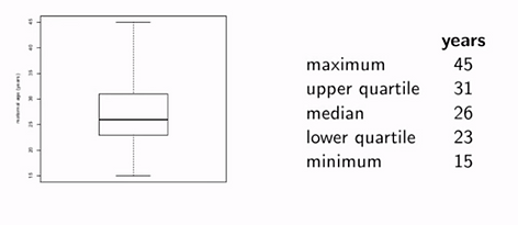
That’s the diagram that shows you
-
maximum of data
-
minimum of data
-
25th percentile (lower Quartile)
-
median
-
75th percentile (upper Quartile)
-

Standard Deviation
(060416)
-
Variance
-
Standard Deviation: How far off are the values or entries from the average?
-
Root mean square of deviation from Average = Square Root of the variance
-
The main thing to take away from the Standard Deviation is:
-
It doesn't matter what the shape of the histogram is.
-
If you've calculated the average and you've calculated the SDs, you can say that the huge chunk of the list is going to be in the range average plus or minus 2, 3, 4 SDs.
-
Chebyshev's Inequality
(060416)
-
That is an amazing boundary for identification of specific entries among all of our data
-
Differences between Markov’s inequality and Chebyshev’s inequality:
-
In Markov’s inequality is not taken into account the SD, hence, it cannot indicate us a precise boundary, whereas in Chebyshev’s inequality we can see with regard to the SD we get a more precise boundary
-
-
Converting to and from Standard Units
-
Z-Score
Section 5:
The normal Curve
(060416)
-
Bell shaped curves; the standard normal curve
-
Normal curves: relation to the standard normal
-
Approximating data histograms; percentiles revisited
-
Not all histograms are bell shaped; Chebyshev revisited
Standard Normal Curve
(060416)
-
A list of some values that are useful for normal distribution:


Section 6:
Relation between two Variables
(060416)
-
Scatter diagrams
-
The correlation coefficient: calculation and properties
-
Using r: with caution!
Scatter Plot
(060416)
-
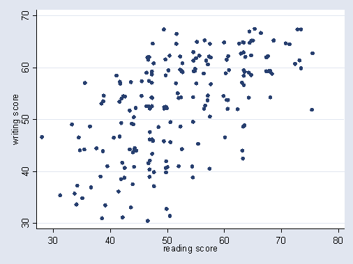
Scatter Plot illustrates linear association
and non-linear association

Association vs. Causation
(060416)
-
Association: that is a technical term for any relation between the variables
-
Correlation coefficient (r) : a number between -1 and 1; it measures LIENAR ASSOCIATION and shows, how tightly the points are clustered about a straight line
-
It doesn’t matter if you switch the variables x and y; r stays the same
-
Association is not causation: If two variables have a non-zero correlation, then they are related to each other in some way, but that doesn’t mean that one causes the other.
Section 7:
Regression
(060416)
-
Estimation; bivariate normal (“football shaped”) scatter diagrams
-
Regression line: intuition; the equation in standard units; regression estimates
-
Regression effect, Galton, and the regression fallacy
-
Equation of the regression line
Football Shaped
(060416)
-
Least squares estimate: average
-
If the scatter diagram is roughly football shaped, you can assume:
-
the distributions of both the variables are roughly normal
-
the distribution of values in each vertical and horizontal strip is roughly normal
-
Regression Line
(060416)
-
Regression Line or Least square: it makes the smallest mean square error among all straight lines. This happens to be true, regardless of the shape of the scatter diagram

Section 8:
Error in the Regression Estimate
(060416)
-
Least squares: why the regression line and no other
-
The r.m.s. error of regression; calculations assuming bivariate normal scatter
-
How regression is commonly used; estimating an “unknown true line”
Error
(060416)
-
Vertical distance between the point and your line
-
Error may be positive (points above the line), negative (points below the line) or zero (points on the line)
-
Rough size of error: r.m.s of the list of errors
-
Residual Plot

Conclusions
(060416)
-
No matter what the scatter diagram is, you can calculate the regression line. That doesn't mean you should use it
-
Never do a regression without first drawing the original scatter plot and at the end drawing a residual plot